Cookbook
All the examples presented below can be found in examples. For the details of each function or class, refer to the API documentation (pyanomaly).
First, import the packages as follows:
import matplotlib.pyplot as plt
from pyanomaly.globals import *
from pyanomaly.fileio import read_from_file
from pyanomaly.characteristics import FUNDA, FUNDQ, CRSPM, CRSPD, Merge
from pyanomaly.jkp import make_factor_portfolios
from pyanomaly.tcost import TransactionCost, TimeVaryingCost
from pyanomaly.analytics import *
from pyanomaly.wrdsdata import WRDS
Example 1
Firm characteristics generation replicating JKP.
This example shows the full process of i) data download, ii) factor creation, and iii) characteristics creation. This example replicates the JKP’s SAS code as closely as possible.
In this example,
funda is merged with fundq to create quarterly updated annual accounting data.
The latest market equity (me) is used when creating firm characteristics.
Generate firm characteristics that appear in the JKP’s paper.
- Note:
Some firm characteristics’ definitions are different from those of JKP’s. To follow JKP’s definitions, set
config.REPLICATE_JKP = True. This will make the program use JKP’s definitions when possible.config.REPLICATE_JKPis only for verification purpose and will be deprecated.
Initialization
Set the log file path and initialize time check (can be skipped).
# Set log file path. Without this, the log will be printed in stdout.
set_log_path('./log/example1.log')
# initialize time check.
elapsed_time('Start of Example 1.')
Data download
Download data frm WRDS.
wrds = WRDS(wrds_username)  # Use your WRDS user id.
# Download all necessary data.
wrds.download_all(run_in_executer=False)  # run_in_executer=True will download faster but consumes more memory.
# Create crspm(d) from m(d)sf and m(d)seall and add gvkey to them.
wrds.preprocess_crsp()
Factor generation
Generate FF3 and HXZ4 factors. These are used in some firm characteristics, such as the residual momentum.
make_factor_portfolios(monthly=True)  # Monthly factors
make_factor_portfolios(monthly=False)  # Daily factors
Characteristic generation
# Generate characteristics in 'jkp' column in mapping.xlsx.
alias = 'jkp'
# Start date. Set to None to create characteristics from as early as possible.
sdate = '1950-01-01'

###################################
# CRSPM
###################################
# Generate firm characteristics from crspm.

crspm = CRSPM(alias=alias)
# Load crspm.
crspm.load_data(sdate)

# Filter data on shrcd, ...
crspm.filter_data()
# Fill missing months by populating the data.
# There are only few missing data and the results aren't affected much by this.
crspm.populate(freq=MONTHLY, method=None)
# Some preprocessing, e.g., creating frequently used variables.
crspm.update_variables()
# Merge crspm with the factors created earlier.
crspm.merge_with_factors()

# Display what characteristics will be generated. Just for information.
crspm.show_available_functions()
# Create characteristics.
crspm.create_chars()

# Postprocessing: delete temporary variables, etc.
crspm.postprocess()
# Saves the results. You can give a file name if you wish. Otherwise, the file name will be the lower-case class
# name, i.e., crspm. The file can later be loaded using the method, crspm.load().
crspm.save()

###################################
# CRSPD
###################################
# Generate firm characteristics from crspd.

crspd = CRSPD(alias=alias)
# Load crspd.
crspd.load_data(sdate)

# Filter data on shrcd, ...
crspd.filter_data()
crspd.update_variables()
crspd.merge_with_factors()

crspd.show_available_functions()
crspd.create_chars()

crspd.postprocess()
crspd.save()

###################################
# FUNDQ
###################################
# Generate firm characteristics from fundq.

fundq = FUNDQ(alias=alias)
# Load fundq.
fundq.load_data(sdate)

# fundq has some duplicates (same datedate/gvkey). Drop duplicates.
fundq.remove_duplicates()
# Convert values in another currency (currently only CAD) to USD values.
fundq.convert_currency()
# Populate data to monthly.
fundq.convert_to_monthly()
# Make quarterly variables from ytd variables and use them to fill missing quarterly variables.
fundq.create_qitems_from_yitems()
fundq.update_variables()

fundq.show_available_functions()
fundq.create_chars()

fundq.postprocess()
fundq.save()

###################################
# FUNDA
###################################
# Generate firm characteristics from funda.

funda = FUNDA(alias=alias)
# Load fundq.
funda.load_data(sdate)

funda.convert_currency()
funda.convert_to_monthly()
# Generate quarterly-updated funda data from fundq and merge them with funda.
funda.merge_with_fundq(fundq)
funda.update_variables()
# Add the market equity of crspm to funda.
funda.add_crsp_me(crspm)

funda.show_available_functions()
funda.create_chars()

funda.postprocess()
funda.save()

###################################
# Merge
###################################
# Combine everything together and generate firm characteristics that require data from multiple data sources.

merge = Merge()
# Merge all data together.
merge.preprocess(crspm, crspd, funda, fundq)

merge.show_available_functions()
merge_chars = merge.get_available_chars()
merge.create_chars(merge_chars)

merge.postprocess()
# By default, `Panel.save()` saves all the columns of `Panel.data`.
# If you want to save only the variables you need to save the disc space, you can do, e.g.:
# columns = ['gvkey', 'datadate', 'primary', 'me', 'ret', 'exret', 'rf']
# merge.save(other_columns=columns)
# Then, all firm characteristics plus the columns in `columns` will be saved.
merge.save()

elapsed_time('End of Example 1.')
Example 2
Different ways of generating characteristics.
This example demonstrates
how to generate a few selected firm characteristics without adding a column to mapping.xlsx;
how to set the output file path instead of the default path.
It is assumed that data has been downloaded from WRDS.
Short-term reversal and 12M-momentum will be generated.
alias is set to None, which means function names are used as aliases.
elapsed_time('Start of Example 2.')

alias = None  # alias = function names
sdate = None  # create characteristics from as early as possible.

# Characteristics to generate: short-term reversal and 12M-momentum.
chars = ['ret_1_0', 'ret_12_1']

# Generate firm characteristics from crspm.
crspm = CRSPM(alias=alias)
crspm.load_data(sdate)

# Filter data on shrcd, ...
crspm.filter_data()
# Let's skip populate() to save time as it doesn't change the result much.
# crspm.populate(freq=MONTHLY, method=None)

# Some preprocessing, e.g., creating frequently used variables.
crspm.update_variables()

# Give a list of characteristics to generate.
crspm.create_chars(chars)

crspm.postprocess()

# Save the output to ./output2/example2.pickle.
# `other_columns=[]` will save only the characterisitcs.
crspm.save('example2', fdir='output2', other_columns=[])

elapsed_time('End of Example 2.')
Example 3
Firm characteristics using year-end ME.
This example demonstrates how to generate funda firm characteristics using year-end ME instead of the latest ME.
All firm characteristics defined in FUNDA are generated.
Only USD-denominated stocks are sampled: currency conversion is unnecessary.
Only funda is used without merging with fundq: merging the two datasets as in Example 1 is also possible.
It is assumed that funda data is available 6 months later.
It is assumed that data has been downloaded from WRDS.
Set variables
alias = None  # Generate all characteristics.
sdate = None  # create characteristics from as early as possible.
Market equity
# Load crspm as we need ME.
crspm = CRSPM(alias=alias)
crspm.load_data(sdate)

# Preprocessing
crspm.filter_data()
crspm.populate(freq=MONTHLY, method=None)

# 'me' and 'me_company' (firm-level me) are generated here.
crspm.update_variables()
Firm characteristics
funda = FUNDA(alias=alias)
funda.load_data(sdate)

# USD stocks only. This is equivalent to funda.data = funda.data[funda.data['curcd'] == 'USD']
funda.filter(('curcd', '==', 'USD'))

funda.convert_to_monthly(lag=6)  # lag=6 means funda is available 6 months later.
funda.update_variables()

# Add year-end market equity to funda.
funda.add_crsp_me(crspm, method='year_end')

# Generate firm characteristics.
funda.show_available_functions()
funda.create_chars()

# Postprocess and save results.
funda.postprocess()
funda.save('funda_eg3')
Example 4
Defining a new characteristic.
This example demonstrates how to define a new class by inheriting CRSPM and add a new characteristic.
A new characteristic, ‘excess_ret_change’, will be added, which is defined as the excess return over the market return divided by the one-year average excess return (I have no idea if this has any predictive power).
It is assumed that data has been downloaded from WRDS.
Defining a new characteristic function
Define a new class by inheriting CRSPM and add a new function c_excess_ret_change() that defines
the new characteristic.
class MyCRSPM(CRSPM):

    # Function for the new characteristic.
    # Note that function name should be of the form 'c_[characteristic name]'.
    def c_excess_ret_change(self):
        """Change of excess return over the market return."""
        # Make a short (one-line) docstring for description.
        # This is displayed when `show_available_functions()` is called.

        cm = self.data

        # One-year average excess return
        avg_exret = self.rolling(cm.exret - cm.mktrf, 12, 'mean')
        # Excess return.
        exret = cm.exret - cm.mktrf

        # Characteristic
        char = exret / avg_exret

        return char
New characteristic generation
alias = None  # alias = function names
sdate = None  # create characteristics from as early as possible.

# Characteristics to generate: the function name is the characteristic name without alias.
chars = ['excess_ret_change']

# Instantiate the class defined above.
crspm = MyCRSPM(alias=alias)
crspm.load_data(sdate)

crspm.filter_data()
crspm.update_variables()

# We need to add factors as we need the market return.
crspm.merge_with_factors()

# Let's see if 'excess_ret_change' has been added.
crspm.show_available_functions()

# Let's create the characteristic!
crspm.create_chars(chars)

crspm.postprocess()
crspm.save('example4')

# Later, you can load the saved file using 'read_from_data()'
data = read_from_file('example4')
print(data['excess_ret_change'])
Example 5
Sorting-based portfolio analysis.
This example demonstrates how to construct quantile portfolios and carry out 1-D or 2-D sorts.
Quintile portfolios will be generated from the 12-month momentum and their mean returns and t-values will be computed.
5x5 2-D sort will be conducted on momentum and size.
Firm-level cross-sectional regression will be conducted.
Factor regressions will be carried out using FF 3-factors.
It is assumed that the firm characteristic has been created and saved to ‘crspm.pickle’.
See also pyanomaly.jkp module for factor and characteristic portfolio creation replicating JKP’s SAS code.
Set variables
char = 'ret_12_1'  # 12-month momentum
char_class = char + '_class'  # Group column: portfolio-stock mapping
ret_col = 'futret'  # Future return column
weight_col = 'me'  # Market equity column
split = 5  # Qintile. You can also do split = [0.2, 0.4, 0.6, 0.8].
labels = ['H', 2, 3, 4, 'L', 'H-L']  # Portfolio names: 'H-L' for long short.
Load data
# Read crspm data (not raw data but the output data).
data = read_from_file('crspm')

# If you want to exclude bottom 20% based on NYSE size...
data['nyse_me'] = np.where(data.exchcd == 1, data[weight_col], np.nan)  # NYSE me
data = filter(data, weight_col, (0.2, None), by='nyse_me')

# Make the future return. If it's already in the data, this step can be skipped.
data[ret_col] = make_future_return(data['exret'])  # Excess return

# Note that the future return at t is the return between t and t+1 and other values are as of t.
# If you want the return at t to be the return between t-1 and t and all other values as of t-1,
# you have to shift forward data as follows.
data = data.groupby(level=-1).shift(1)  # Shift data forward.
data = data.dropna(subset=[ret_col])  # Drop nan returns.
1-D sort
# Classify stocks based on char.
data[char_class] = classify(data[char], split, ascending=False)

# Make quantile portfolios.
# qpfs will have index = date/classes and columns = ['futret']
qpfs = one_dim_sort(data, char_class, ret_col, weight_col=weight_col)

# You can add more columns to the portfolios. Here I add `signal` (mean of the characteristic) and
# n_firms (number of firms).
qpfs[['signal', 'n_firms']] = one_dim_sort(data, char_class, char, function=['mean', 'count'])

# If you want to see the average size and price of the portfolios...
qpfs[['size', 'prc']] = one_dim_sort(data, char_class, [weight_col, 'prc'])

# Name the portfolios. Without this, the names are 0, 1, ...
relabel_class(qpfs, labels)

print(f'Quantile portfolios sorted on {char}')
print(qpfs)

# Calculate the time-series mean and t-value of the future return for each portfolio.
# avg and tval have index values equal to the portfolio names.
avg, tval = time_series_average(qpfs[ret_col], cov_type='HAC', cov_kwds={'maxlags': 12})
print(f'\n Mean of portfolio returns sorted on {char}')
print(avg)
print(tval)
# Put them together to make a nice table.
print(pd.concat([avg, tval], axis=1, keys=['mean', 't-val']))
Output:
Quantile portfolios sorted on ret_12_1
                           futret  signal  n_firms      size     prc
date       ret_12_1_class
1927-01-31 H               -0.010   0.482       69    85.210  73.924
           2                0.009   0.151       69   131.678  89.196
           3               -0.001   0.013       69    91.500  83.021
           4               -0.004  -0.106       69    54.869  54.849
           L               -0.005  -0.329       69    25.706  34.803
           H-L             -0.005   0.811        0    59.504  39.120
1927-02-28 H                0.055   0.442       71    97.356  81.886
           2                0.040   0.151       70   130.918  89.640
           3                0.028   0.048       71    77.347  74.449
           4                0.048  -0.074       70    55.549  52.839
           L                0.067  -0.299       71    26.083  34.153
           H-L             -0.012   0.741        0    71.273  47.732
                           ...     ...      ...       ...     ...
2020-12-31 H                0.057   1.188      442 27538.688 118.659
           2                0.024   0.174      442 23863.618 115.923
           3                0.038  -0.042      442 20827.442 867.161
           4                0.066  -0.208      442 11994.607  70.635
           L                0.070  -0.444      442  6082.012  34.062
           H-L             -0.013   1.631        0 21456.676  84.597

 Mean of portfolio returns sorted on ret_12_1
ret_12_1_class
H     0.012
2     0.008
3     0.007
4     0.006
L     0.005
H-L   0.007
Name: futret, dtype: float64
ret_12_1_class
H     5.836
2     4.989
3     3.864
4     3.393
L     2.006
H-L   4.215
Name: futret, dtype: float64
                mean  t-val
ret_12_1_class
H              0.012  5.836
2              0.008  4.989
3              0.007  3.864
4              0.006  3.393
L              0.005  2.006
H-L            0.007  4.215
2-D sort
# Let's make a 5x5 portfolios on char and char2.
char2 = 'me'
char_class2 = char2 + '_class'
split2 = 5
labels2 = ['S', 2, 3, 4, 'B', 'S-B']

# Classify stocks based on char2 in ascending order.
data[char_class2] = classify(data[char2], split2, ascending=True)

# Make 5x5 portfolios.
# qpfs2 will have index = date/char_class/char_class2 and columns = ['futret'].
qpfs2 = two_dim_sort(data, char_class, char_class2, ret_col, weight_col=weight_col)

# Make char_class2 as columns. Now columns are ['S', 2, 3, 4, 'B', 'S-B']
qpfs2 = qpfs2.unstack()
qpfs2.columns = qpfs2.columns.droplevel(0)

# Name the portfolios. We relabel after unstacking as `unstack()` sort values.
relabel_class(qpfs2, labels)
relabel_class(qpfs2, labels2, axis=1)

# Calculate the time-series mean and t-value of the future return for each portfolio.
avg, tval = time_series_average(qpfs2, cov_type='HAC', cov_kwds={'maxlags': 12})
print(f'\n Mean of portfolio returns sorted on {char} and {char2}')
print(avg)
print(tval)
Output:
 Mean of portfolio returns sorted on ret_12_1 and me
me_class           S     2     3     4     B    S-B
ret_12_1_class
H              0.035 0.016 0.014 0.013 0.010  0.025
2              0.027 0.011 0.010 0.010 0.008  0.019
3              0.025 0.010 0.009 0.008 0.006  0.019
4              0.024 0.009 0.007 0.007 0.006  0.018
L              0.030 0.006 0.005 0.005 0.003  0.027
H-L            0.005 0.010 0.009 0.008 0.007 -0.002
me_class            S     2     3     4     B    S-B
ret_12_1_class
H              11.994 6.911 6.089 5.887 5.109 10.926
2               9.127 5.415 4.613 5.342 4.725  8.555
3               9.143 4.843 4.072 4.148 3.585  9.163
4               8.261 3.857 3.242 3.303 3.322  9.258
L               8.391 2.211 1.796 1.974 1.405 10.429
H-L             2.293 5.520 5.356 4.905 4.077 -1.411
Firm-level cross-sectional regression
Regress return cross-sectionally on the t-1 characteristic and other variables at each date t. Take the time-series average of the coefficients and examine their significance.
# X: For simplicity, we will only use the characteristic and the size.
exog_cols = [char, 'me']

# Run the regressions. This function returns the average coefficients, t-values, and coefficients time-series.
avg, tval, coef = crosssectional_regression(data, ret_col, exog_cols, add_constant=True, cov_type='HAC',
                                            cov_kwds={'maxlags': 12})
print('\nMean of the coefficients')
print(pd.concat([avg, tval], axis=1))
print('\nCoefficients time-series')
print(coef)
Output:
Mean of the coefficients
           mean  t-stat
const     0.012   5.838
ret_12_1  0.007   4.177
me       -0.000  -2.450

Coefficients time-series
            const  ret_12_1     me
1927-01-31  0.015     0.005 -0.000
1927-02-28  0.064    -0.018 -0.000
1927-03-31 -0.025     0.046  0.000
1927-04-30 -0.012     0.050  0.000
           ...       ...    ...
2020-09-30 -0.031     0.012 -0.000
2020-10-31  0.028    -0.013 -0.000
2020-11-30  0.194     0.008 -0.000
2020-12-31  0.087    -0.013 -0.000
Factor regression
Regress quantile portfolios’ returns on the FF-3 factors.
# Sample period.
sdate = '1952-01'
edate = '2020-12'

qpfs = qpfs[sdate:edate]

# Read factors.
# Here I use the factors generated by PyAnomaly. You can use different sources if you like.
factors = read_from_file(config.factors_monthly_fname)
# factors = WRDS.read_data('factors_monthly')  # factors from K.French website.

# X: Constant + FF3.
X = factors.loc[sdate:edate, ['mktrf', 'smb_ff', 'hml']].values
# X = factors.loc[sdate:edate, ['mktrf', 'smb', 'hml']].values  # If you use K. French data.
X = sm.add_constant(X)

# Run the regression for each portfolio.
result = {}
for pf in qpfs.index.get_level_values(-1):
    # y: Returns of a portfolio
    y = qpfs.loc[(slice(None), pf), 'futret'].values

    model = sm.OLS(y, X).fit()

    # Make an output table.
    result[pf] = pd.DataFrame({'coefs': model.params, 'tval': model.tvalues}, index=['const', 'mktrf', 'smb', 'hml'])

result = pd.concat(result, axis=1)
print('\nFactor regression: FF3')
print(result)
Output:
Factor regression: FF3
           H              2             3             4             L           H-L
       coefs    tval  coefs   tval  coefs   tval  coefs   tval  coefs   tval  coefs    tval
const  0.005   7.125  0.002  3.685  0.000  0.925 -0.001 -2.154 -0.005 -5.758  0.011   7.424
mktrf  1.028  56.623  0.964 79.587  0.951 87.918  1.004 77.950  1.223 56.655 -0.195  -5.705
smb    0.201   7.141 -0.111 -5.907 -0.093 -5.537 -0.028 -1.423  0.258  7.718 -0.057  -1.082
hml   -0.479 -22.131 -0.097 -6.720  0.100  7.717  0.312 20.317  0.587 22.812 -1.066 -26.172
Example 6
Quantile portfolio construction and performance evaluation.
This example demonstrates how to construct quantile portfolios (and the long-short) based on a firm characteristic and evaluate their performance.
Tercile portfolios will be generated from the 12-month momentum.
Different ways of setting the transaction cost will shown.
It is assumed that the firm characteristic has been created and saved to ‘crspm.pickle’.
Set variables
char = 'ret_12_1'  # 12-month momentum
char_class = char + '_class'  # Group column: portfolio-stock mapping
ret_col = 'futret'  # Future return column
weight_col = 'me'  # Market equity column
split = 3  # Tercile. You can also do split = [0.2, 0.8] for 2:6:2 split.
labels = ['H', 'M', 'L', 'H-L']  # Portfolio names: 'H-L' for long short.
Load data
# Read crspm data (not raw data but the output data).
data = read_from_file('crspm')

# NYSE me
data['nyse_me'] = np.where(data.exchcd == 1, data[weight_col], np.nan)

# Make the future return. If it's already in the data, this step can be skipped.
data[ret_col] = make_future_return(data['ret'])

# Let's just keep the data we need. Below is the same as `data = data[[char, ret_col, weight_col]]`
# but faster and more memroy efficient.
keep_columns(data, [char, ret_col, weight_col])

# Risk-free rates.
# Don't forget to set `month_end=True` since the crspm date has also been shifted to month end.
rf = WRDS.get_risk_free_rate(month_end=True)
Transaction costs
PyAnomaly provides a powerful way to set transaction costs via TransactionCost class.
See pyanomaly.tcost module for details.
Below are some examples of setting transaction costs.
# No transaction costs.
costfcn = None

# Transaction cost of 30 basis points.
costfcn = 0.003

# 20 (30) bps when buying (selling).
costfcn = TransactionCost(buy_linear=0.002, sell_linear=0.002)
In this example, we will assume transaction cost that decreases over time and with size.
costfcn = TimeVaryingCost(data[weight_col])
Portfolio construction
In PyAnomaly, Portfolio class is used to make a portfolio from position information.
The make_position() function converts a panel data to position data that is used as the input to Portfolio class.
In the panel data, the future return at t is the return between t and t+1, whereas in the position data, dates are shifted
so that the future return at t is the return between t-1 and t.
# Here, we remove small-cap stocks after setting the cost function.
# This is because `TimeVaryingCost` requires all firms' me as the input.
data = filter(data, weight_col, (0.2, None), by='nyse_me')

# Classify data on char. The highest momentum stock will be labeled 0 and the lowest 2.
data[char_class] = classify(data[char], split, ascending=False)

# Make position data.
# Set weight_col = None for equally-weighted portfolios.
# `other_cols` are the columns you want to keep in the position data.
position = make_position(data, ret_col, weight_col, char_class, other_cols=None)

# Make portfolios. `portfolios` will have four portfolios, 'H', 'M', 'L', and 'H-L'.
portfolios = make_quantile_portfolios(position, char_class, rf=rf, costfcn=costfcn, labels=labels)
Performance evaluation
Portfolios can be evaluated using Portfolio.eval() for a single portfolio or Portfolios.eval() for a
collection of portfolios.
# `annualize_factor=12` will annualize the results as crspm is monthly data.
pfperfs, pfvals = portfolios.eval(annualize_factor=12)

# Performance metrics.
print('\nPerformance')
print(pfperfs)

# Time-series of portfolio value, return, ...
print('\nValues')
print(pfvals)
Output:
Performance
                    H           M           L         H-L
mean            0.042      -0.032      -0.029      -0.114
std             0.195       0.190       0.247       0.167
sharpe          0.215      -0.170      -0.118      -0.681
cum             5.176      -1.661      -2.466     -12.287
mdd             0.818       0.985       0.990       1.000
mdd start  1929-08-31  1929-08-31  1929-01-31  1932-06-30
mdd end    1942-04-30  1982-07-31  1982-07-31  2020-12-31
msd             0.422       0.505       0.608       0.784
msd start  1937-07-31  1932-02-29  1932-02-29  1932-06-30
msd end    1938-01-31  1932-06-30  1932-06-30  1932-09-30
turnover        5.614       7.738       6.260      12.263
lposition     456.613     458.740     458.704     456.613
sposition       0.000       0.000       0.000     458.704

Values
              ret  exret       val1        val lposition sposition    cost tover netret grossret netexret grossexret cumret drawdown drawdur  drawstart succdown succdur  succstart
                H      H          H          H         H         H       H     H      H        H        H          H      H        H       H          H        H       H          H
1927-01-31  0.001 -0.002      1.001      1.000       120     0.000   0.000 0.000  0.001    0.001   -0.002     -0.002  0.001    0.000   0.000 1927-01-31    0.000   0.000 1927-01-31
1927-02-28  0.041  0.039      1.050      1.001       122     0.000   0.008 0.415  0.041    0.049    0.039      0.046  0.041    0.000   0.000 1927-02-28    0.000   0.000 1927-02-28
1927-03-31  0.010  0.007      1.073      1.050       123     0.000   0.013 0.720  0.010    0.022    0.007      0.019  0.051    0.000   0.000 1927-03-31    0.000   0.000 1927-03-31
           ...    ...        ...        ...       ...       ...     ...   ...    ...      ...      ...        ...    ...      ...     ...        ...      ...     ...        ...    ...
2020-10-31 -0.028 -0.028 246929.635 253650.609       726     0.000 280.481 0.197 -0.028   -0.026   -0.028     -0.027  5.039    0.077   2.000 2020-08-31    0.077   2.000 2020-08-31
2020-11-30  0.101  0.101 272302.967 246929.635       727     0.000 310.721 0.222  0.101    0.103    0.101      0.103  5.135    0.000   0.000 2020-11-30    0.000   0.000 2020-11-30
2020-12-31  0.041  0.041 283833.135 272302.967       736     0.000 306.903 0.197  0.041    0.042    0.041      0.042  5.176    0.000   0.000 2020-12-31    0.000   0.000 2020-12-31
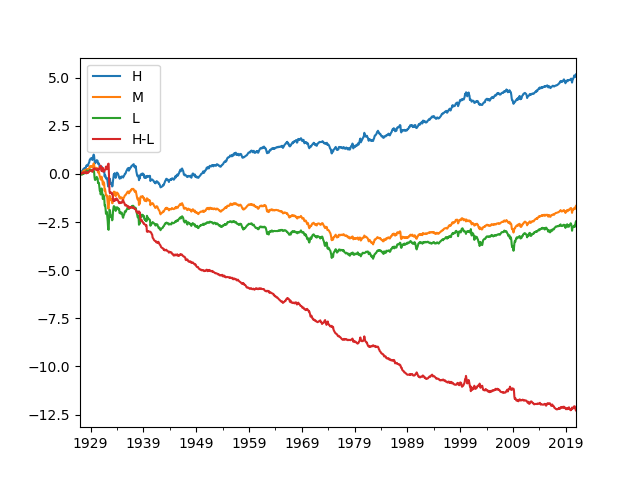
Let’s plot cumulative returns.
pfvals['cumret'].plot()
plt.show()
Output:
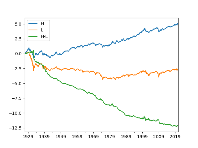
You can also plot selected portfolios.
pfvals['cumret'][['H', 'L', 'H-L']].plot()
plt.show()
Output:
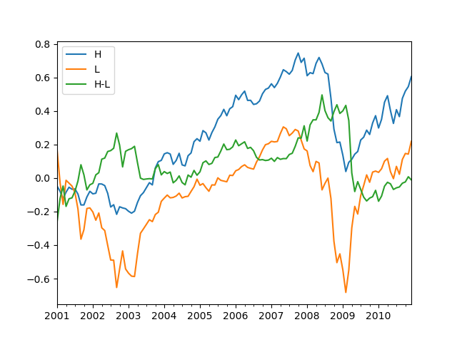
You can evaluate the portfolios for a sub-period and choose to ignore transaction costs.
pfperfs1, pfvals1 = portfolios.eval(sdate='2001-01-01', edate='2010-12-31', annualize_factor=12, consider_cost=False)
print('\nPerformance: 2001-01 - 2010-12')
print(pfperfs1)
pfvals1['cumret'][['H', 'L', 'H-L']].plot()
plt.show()
Output:
Performance: 2001-01 - 2010-12
                    H           M           L         H-L
mean            0.054       0.023       0.033       0.020
std             0.169       0.149       0.256       0.201
sharpe          0.318       0.154       0.130       0.102
cum             0.605       0.330       0.219      -0.011
mdd             0.507       0.447       0.628       0.470
mdd start  2007-10-31  2007-10-31  2007-05-31  2008-06-30
mdd end    2009-02-28  2009-02-28  2009-02-28  2010-01-31
msd             0.398       0.255       0.396       0.402
msd start  2008-05-31  2008-08-31  2008-08-31  2009-02-28
msd end    2008-11-30  2008-11-30  2008-11-30  2009-05-31
turnover        6.308       7.591       6.138      12.930
lposition     669.283     673.458     672.458     669.283
sposition       0.000       0.000       0.000     672.458
You can access one of the portfolios, evaluate it, and view its position details.
# To access portfolio 'H'
pf_h = portfolios['H']
pf_h_perf, pf_h_val = pf_h.eval()  # no annualize

# You can also access the returns of `eval()` as follows.
print('\nPerformance: H')
print(pf_h.performance)  # pf_h_perf
print('\nValues: H')
print(pf_h.value)  # pf_h_val

# To see the positions (constituents)
print('\nPositions: H')
print(pf_h.position)
Output:
Performance: H
                    H
mean            0.004
std             0.056
sharpe          0.062
cum             5.176
mdd             0.818
mdd start  1929-08-31
mdd end    1942-04-30
msd             0.422
msd start  1937-07-31
msd end    1938-01-31
turnover        0.468
lposition     456.613
sposition       0.000

Values: H
              ret  exret       val1        val  lposition  sposition    cost  tover  netret  grossret  netexret  grossexret  cumret  drawdown  drawdur  drawstart  succdown  succdur  succstart
1927-01-31  0.001 -0.002      1.001      1.000        120      0.000   0.000  0.000   0.001     0.001    -0.002      -0.002   0.001     0.000    0.000 1927-01-31     0.000    0.000 1927-01-31
1927-02-28  0.041  0.039      1.050      1.001        122      0.000   0.008  0.415   0.041     0.049     0.039       0.046   0.041     0.000    0.000 1927-02-28     0.000    0.000 1927-02-28
1927-03-31  0.010  0.007      1.073      1.050        123      0.000   0.013  0.720   0.010     0.022     0.007       0.019   0.051     0.000    0.000 1927-03-31     0.000    0.000 1927-03-31
           ...    ...        ...        ...        ...        ...     ...    ...     ...       ...       ...         ...     ...       ...      ...        ...       ...      ...        ...
2020-10-31 -0.028 -0.028 246929.635 253650.609        726      0.000 280.481  0.197  -0.028    -0.026    -0.028      -0.027   5.039     0.077    2.000 2020-08-31     0.077    2.000 2020-08-31
2020-11-30  0.101  0.101 272302.967 246929.635        727      0.000 310.721  0.222   0.101     0.103     0.101       0.103   5.135     0.000    0.000 2020-11-30     0.000    0.000 2020-11-30
2020-12-31  0.041  0.041 283833.135 272302.967        736      0.000 306.903  0.197   0.041     0.042     0.041       0.042   5.176     0.000    0.000 2020-12-31     0.000    0.000 2020-12-31

Positions: H
               id    ret   wgt    rf  exret      val     val1     val0   cost
date
1927-01-31  10049 -0.027 0.004 0.002 -0.030    0.004    0.003    0.004  0.000
1927-01-31  10102 -0.018 0.002 0.002 -0.020    0.002    0.002    0.002  0.000
1927-01-31  10129 -0.007 0.003 0.002 -0.009    0.003    0.003    0.003  0.000
           ...    ...   ...   ...    ...      ...      ...      ...    ...
2020-12-31  93369  0.184 0.000 0.000  0.184   32.099   38.018   31.771  0.002
2020-12-31  93393  0.092 0.000 0.000  0.092   13.010   14.207   12.877  0.001
2020-12-31  93436  0.243 0.027 0.000  0.243 7299.521 9075.147 7225.128  0.391
Example 7
New table download.
This example demonstrates how to download a new table from WRDS. Different ways of downloading comp.secm table are demonstrated.
Connect to WRDS.
wrds = WRDS(wrds_usename)
Method 1: Download the entire table at once.
wrds.download_table('comp', 'secm', date_cols=['datadate']) # 'datadate's type will be converted to datetime.
Method 2: Download the entire table asynchronously.
This downloads data every interval years along date_col. This is a memory efficient way of downloading a large dataset.
For a small size data, this can be slower than download_table().
wrds.download_table_async('comp', 'secm', date_col='datadate', date_cols=['datadate'], interval=5)
Method 3: Download only some fields.
sql = 'datadate, gvkey, cshoq, prccm'
wrds.download_table_async('comp', 'secm', sql=sql, date_col='datadate', date_cols=['datadate'])
Method 4: Download data using a complete query statement.
Below is equivalent to the above. Note that the query statement must contain ‘WHERE [date_col] BETWEEN {} and {}’.
sql = f"""
    SELECT datadate, gvkey, cshoq, prccm
    FROM comp.secm
    WHERE datadate between '{{}}' and '{{}}'
"""
wrds.download_table_async('comp', 'secm', sql=sql, date_cols=['datadate'])